GDAS008-IRanges和GRanges

前言

原始的Rmd文档可以参考Github上。

IRangesGRanges 对象是Bioconductor基础数据类型的核心成员,其中 IRanges 定义了 integer ranges ,它用于解决基因组上的位置问题,而 GRanges 则包含了染色体和DNA链的信息。这里我们简介绍一下这两个对象,以及如何操作 IRangesGRanges

IRanges

第一步是加载IRanges包,如下所示:

1
library(IRanges)

IRanges 函数定义了区间范围(interval ranges)。如果你输入2个数据,那么就表示一个区间,例如 [5,10]={5,6,7,8,9,10},它的宽度是6。另外,如果我们要查看一个 IRanges 定义的区间宽度,我们使用的width()函数,而非 length()函数,如下所示:

1
2
3
4
5
6
7
8
9
10
11
12
13
14
15
16
ir <- IRanges(5,10)
ir
## IRanges object with 1 range and 0 metadata columns:
## start end width
## <integer> <integer> <integer>
## [1] 5 10 6
start(ir)
## [1] 5
end(ir)
## [1] 10
width(ir)
## [1] 6
# for detailed information on the IRanges class:
# ?IRanges
length(ir)
# [1] 1

一个单独的IRanges对象可以含有多个范围。现在我们可以在一个向量中指定start,在另外一个向量中指定end,如下所示:

1
2
3
4
5
6
7
IRanges(start=c(3,5,17), end=c(10,8,20))
## IRanges object with 3 ranges and 0 metadata columns:
## start end width
## <integer> <integer> <integer>
## [1] 3 10 8
## [2] 5 8 4
## [3] 17 20 4

内部范围(Intra-range)操作

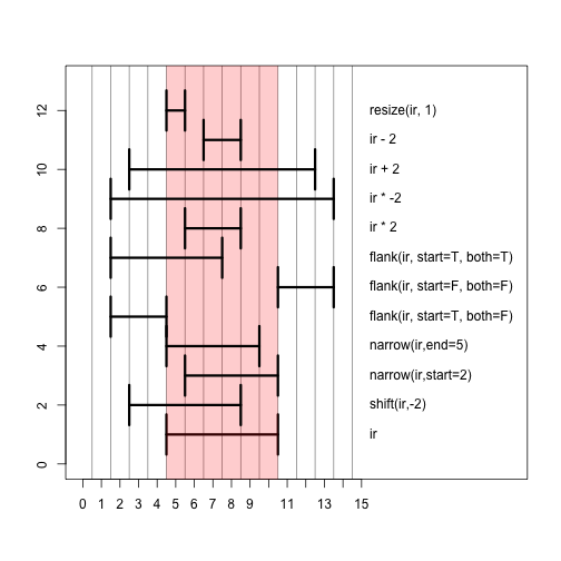
现在我们继续使用单个范围[5,10],我们查看内部范围(intra-range){…,−2,−1,0,1,2,…}的一个数,如下所示:

1
2
3
4
5
6
7
8
9
10
11
12
# full details on the intra-range methods:
# ?"intra-range-methods"
ir
## IRanges object with 1 range and 0 metadata columns:
## start end width
## <integer> <integer> <integer>
## [1] 5 10 6
shift(ir, -2)
## IRanges object with 1 range and 0 metadata columns:
## start end width
## <integer> <integer> <integer>
## [1] 3 8 6

这里我们展示了应用于ir的多个不同操作的结果,结果如下所示:

1
2
3
4
5
6
7
8
9
10
11
12
13
14
15
16
17
18
19
20
21
22
23
24
25
26
27
28
29
30
31
32
33
34
35
36
37
38
39
40
41
42
43
44
45
46
47
48
49
50
51
52
53
54
55
ir
## IRanges object with 1 range and 0 metadata columns:
## start end width
## <integer> <integer> <integer>
## [1] 5 10 6
narrow(ir, start=2)
## IRanges object with 1 range and 0 metadata columns:
## start end width
## <integer> <integer> <integer>
## [1] 6 10 5
narrow(ir, end=5)
## IRanges object with 1 range and 0 metadata columns:
## start end width
## <integer> <integer> <integer>
## [1] 5 9 5
flank(ir, width=3, start=TRUE, both=FALSE)
## IRanges object with 1 range and 0 metadata columns:
## start end width
## <integer> <integer> <integer>
## [1] 2 4 3
flank(ir, width=3, start=FALSE, both=FALSE)
## IRanges object with 1 range and 0 metadata columns:
## start end width
## <integer> <integer> <integer>
## [1] 11 13 3
flank(ir, width=3, start=TRUE, both=TRUE)
## IRanges object with 1 range and 0 metadata columns:
## start end width
## <integer> <integer> <integer>
## [1] 2 7 6
ir * 2
## IRanges object with 1 range and 0 metadata columns:
## start end width
## <integer> <integer> <integer>
## [1] 6 8 3
ir * -2
## IRanges object with 1 range and 0 metadata columns:
## start end width
## <integer> <integer> <integer>
## [1] 2 13 12
ir + 2
## IRanges object with 1 range and 0 metadata columns:
## start end width
## <integer> <integer> <integer>
## [1] 3 12 10
ir - 2
## IRanges object with 1 range and 0 metadata columns:
## start end width
## <integer> <integer> <integer>
## [1] 7 8 2
resize(ir, 1)
## IRanges object with 1 range and 0 metadata columns:
## start end width
## <integer> <integer> <integer>
## [1] 5 5 1

我们使用下图展示了上面操作的结果。红色柱状部分显示了最初的ir范围。掌握这些操作的最好方法是在自己定义的范围内在控制台中亲自操作一下。

plot of chunk unnamed-chunk-6

内部范围方法

针对intra-range有着一系列的方法。还有一些方法是针对一系列范围的操作,它的输出取决于所有的范围,因此这些方法与intra-range方法不同,后者不会改变输出。现在我们一些案例来说明一下。range()函数提供了从最左侧到最右侧的整数输出,如下所示:

注:原文我不太理解,翻译的不精准,原文如下:

There are also a set of inter-range methods. These are
operations which work on a set of ranges, and the output depends on all
the ranges, thus distinguishes these methods from the intra-range methods, for which the other ranges in the set do not change the output. This is best explained with some examples. The range function gives the integer range from the start of the leftmost range to the end of the rightmost range:

1
2
3
4
5
6
7
8
9
10
11
12
13
14
# full details on the inter-range methods:
# ?"inter-range-methods"
(ir <- IRanges(start=c(3,5,17), end=c(10,8,20)))
## IRanges object with 3 ranges and 0 metadata columns:
## start end width
## <integer> <integer> <integer>
## [1] 3 10 8
## [2] 5 8 4
## [3] 17 20 4
range(ir)
## IRanges object with 1 range and 0 metadata columns:
## start end width
## <integer> <integer> <integer>
## [1] 3 20 18

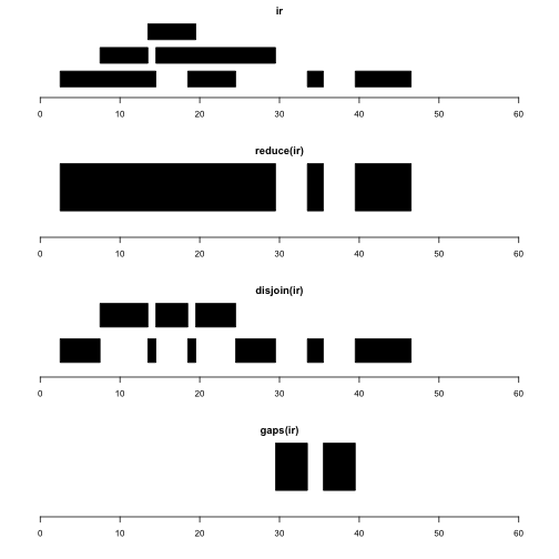
reduce 函数能折叠这些范围,以便于整个可以只被输出范围中的一个范围覆盖,如下所示:

1
2
3
4
5
6
reduce(ir)
## IRanges object with 2 ranges and 0 metadata columns:
## start end width
## <integer> <integer> <integer>
## [1] 3 10 8
## [2] 17 20 4

注:ir原来有3个范围,其中[5,8]范围是在[3,10]之间,因此前者被折叠到了后者之中。

gaps 函数能够给出上面两个范围的区间,但是它不覆盖任何ir中的范围,如下所示:

1
2
3
4
5
gaps(ir)
## IRanges object with 1 range and 0 metadata columns:
## start end width
## <integer> <integer> <integer>
## [1] 11 16 6

disjoin 会打断 ir的范围,并它们分成不同的范围,如下所示:

disjoin返回一个disjoint对象,它会查看参数中端点的并集,返回不相交的对象。换话句讲,结果中由区间的最大长度范围组成,在该范围上,对象x中的重叠范围集合是相同的,并且至少为1。

1
2
3
4
5
6
7
8
disjoin(ir)
## IRanges object with 4 ranges and 0 metadata columns:
## start end width
## <integer> <integer> <integer>
## [1] 3 4 2
## [2] 5 8 4
## [3] 9 10 2
## [4] 17 20 4

现在我们使用示意图来说明一下:

第一二行是原始的范围,第四行是经过disjoin处理后的范围。

GRanges

GRanges对象包含了Iranges,它含有2个方面的重要信息:

  • 染色体信息(Bioconductor称为 seqnames)。
  • DNA链。

链的信息可以指定为 + 号或 - ,或者是保留未指定的 * 。正义链的特征则是在编号线上从左到右的生物学方面,而负链特征则是从右到左。就IRanges而言,正链特征是从startend ,负链则是从 endstart 。这初看起来比较混乱,但这是必需的,因此 width 被定义为 end - start + 1,并且不允许有负的宽度范围。因为DNA有两条链,这两条链具有相反的方向性,因此当我们说DNA时,可以只指明其中的一条链。

通过IRnage、染色体名称和一条链,我们可以确定我们与另外一个研究人员所指的DNA分子具有相同的区域和链,因为我们使用的相同的基因组构建的。GRanges对象中还可以包括其它部分的信息,不过上述的两个信息则是最重要的 。

1
library(GenomicRanges)

现在我们创建一个虚构染色体chrZ 上的两个范围。我们会说这两个范围指的基因组hg19上的范围。因为我们没有将我们的基因组链接到数据库,因此我们可以指定一个在hg19中并不存在的染色体,如下所示:

1
2
3
4
5
6
7
8
9
10
11
12
13
14
15
16
17
18
19
gr <- GRanges("chrZ", IRanges(start=c(5,10),end=c(35,45)),
strand="+", seqlengths=c(chrZ=100L))
gr
## GRanges object with 2 ranges and 0 metadata columns:
## seqnames ranges strand
## <Rle> <IRanges> <Rle>
## [1] chrZ [ 5, 35] +
## [2] chrZ [10, 45] +
## -------
## seqinfo: 1 sequence from an unspecified genome
genome(gr) <- "hg19"
gr
## GRanges object with 2 ranges and 0 metadata columns:
## seqnames ranges strand
## <Rle> <IRanges> <Rle>
## [1] chrZ [ 5, 35] +
## [2] chrZ [10, 45] +
## -------
## seqinfo: 1 sequence from hg19 genome

我们可以调用 seqnamesseqlengths 来查看上面的信息:

1
2
3
4
5
6
7
8
seqnames(gr)
## factor-Rle of length 2 with 1 run
## Lengths: 2
## Values : chrZ
## Levels(1): chrZ
seqlengths(gr)
## chrZ
## 100

我们可以使用 shift 函数(就像在IRanges中使用的一样)来处理GRanges。但是,当我们尝试超过染色体长度之外的范围时,就会出现警告信息,如下所示:

1
2
3
4
5
6
7
8
9
10
11
12
13
14
15
16
17
18
19
20
21
22
23
shift(gr, 10)
## GRanges object with 2 ranges and 0 metadata columns:
## seqnames ranges strand
## <Rle> <IRanges> <Rle>
## [1] chrZ [15, 45] +
## [2] chrZ [20, 55] +
## -------
## seqinfo: 1 sequence from hg19 genome
shift(gr, 80)
## Warning in valid.GenomicRanges.seqinfo(x, suggest.trim = TRUE): GRanges object contains 2 out-of-bound ranges located on sequence
## chrZ. Note that only ranges located on a non-circular sequence
## whose length is not NA can be considered out-of-bound (use
## seqlengths() and isCircular() to get the lengths and circularity
## flags of the underlying sequences). You can use trim() to trim
## these ranges. See ?`trim,GenomicRanges-method` for more
## information.
## GRanges object with 2 ranges and 0 metadata columns:
## seqnames ranges strand
## <Rle> <IRanges> <Rle>
## [1] chrZ [85, 115] +
## [2] chrZ [90, 125] +
## -------
## seqinfo: 1 sequence from hg19 genome

如果我们使用 trim 处理这个范围,我们就能获取剩下的范围,而不考虑超出染色体长的部分:

1
2
3
4
5
6
7
8
9
10
11
12
13
14
15
trim(shift(gr, 80))
## Warning in valid.GenomicRanges.seqinfo(x, suggest.trim = TRUE): GRanges object contains 2 out-of-bound ranges located on sequence
## chrZ. Note that only ranges located on a non-circular sequence
## whose length is not NA can be considered out-of-bound (use
## seqlengths() and isCircular() to get the lengths and circularity
## flags of the underlying sequences). You can use trim() to trim
## these ranges. See ?`trim,GenomicRanges-method` for more
## information.
## GRanges object with 2 ranges and 0 metadata columns:
## seqnames ranges strand
## <Rle> <IRanges> <Rle>
## [1] chrZ [85, 100] +
## [2] chrZ [90, 100] +
## -------
## seqinfo: 1 sequence from hg19 genome

我们可以使用 mcols 函数(链表示元数据列)向每个范围添加列信息。需要注意的是,这个操作对IRanges也是可行的。我们还可以通过指定 NULL 来移除列信息,如下所示:

1
2
3
4
5
6
7
8
9
10
11
12
13
14
15
16
17
18
19
20
mcols(gr)
## DataFrame with 2 rows and 0 columns
mcols(gr)$value <- c(-1,4)
gr
## GRanges object with 2 ranges and 1 metadata column:
## seqnames ranges strand | value
## <Rle> <IRanges> <Rle> | <numeric>
## [1] chrZ [ 5, 35] + | -1
## [2] chrZ [10, 45] + | 4
## -------
## seqinfo: 1 sequence from hg19 genome
mcols(gr)$value <- NULL
> gr
# GRanges object with 2 ranges and 0 metadata columns:
# seqnames ranges strand
# <Rle> <IRanges> <Rle>
# [1] chrZ 5-35 +
# [2] chrZ 10-45 +
# -------
# seqinfo: 1 sequence from hg19 genome

GRangesList

当我们涉及基因时,我们通过创建一个GRanges列表是很有用的,例如用于表示分组信息(比如每个基因的外显子)。该列表的元素是基因,并且在每个元素中,外显子的范围被定义为GRanges。

1
2
3
4
5
6
7
8
9
10
11
12
13
14
15
16
17
18
19
20
gr2 <- GRanges("chrZ",IRanges(11:13,51:53))
grl <- GRangesList(gr, gr2)
grl
## GRangesList object of length 2:
## [[1]]
## GRanges object with 2 ranges and 0 metadata columns:
## seqnames ranges strand
## <Rle> <IRanges> <Rle>
## [1] chrZ [ 5, 35] +
## [2] chrZ [10, 45] +
##
## [[2]]
## GRanges object with 3 ranges and 0 metadata columns:
## seqnames ranges strand
## [1] chrZ [11, 51] *
## [2] chrZ [12, 52] *
## [3] chrZ [13, 53] *
##
## -------
## seqinfo: 1 sequence from hg19 genome

GRangesList 对象中的长度就是其中的GRanges 对象个数。为了获取每个GRanges的长度,我们可以调用 elementNROWS。我们可以通过两个方括号的典型列表索引方法来建立索引,如下所示:

1
2
3
4
5
6
7
8
9
10
11
12
length(grl)
## [1] 2
elementNROWS(grl)
## [1] 2 3
grl[[1]]
## GRanges object with 2 ranges and 0 metadata columns:
## seqnames ranges strand
## <Rle> <IRanges> <Rle>
## [1] chrZ [ 5, 35] +
## [2] chrZ [10, 45] +
## -------
## seqinfo: 1 sequence from hg19 genome

width函数会返回一个 integerList。如果使用sum,我们会得到列表中每个GRanges对象的宽度向量,如下所示:

1
2
3
4
5
6
width(grl)
## IntegerList of length 2
## [[1]] 31 36
## [[2]] 41 41 41
sum(width(grl))
## [1] 67 123

我们可以像以前那样添加元数据(metadata),现在每个GRange对象都有一行元数据。当我们输出GRangesList时它们并不业显示出来,但我们可以通过 mcols 进行访问,如下所示:

1
2
3
4
5
6
7
8
9
10
11
12
13
14
15
16
17
18
19
20
21
22
23
24
25
mcols(grl)$value <- c(5,7)
grl
## GRangesList object of length 2:
## [[1]]
## GRanges object with 2 ranges and 0 metadata columns:
## seqnames ranges strand
## <Rle> <IRanges> <Rle>
## [1] chrZ [ 5, 35] +
## [2] chrZ [10, 45] +
##
## [[2]]
## GRanges object with 3 ranges and 0 metadata columns:
## seqnames ranges strand
## [1] chrZ [11, 51] *
## [2] chrZ [12, 52] *
## [3] chrZ [13, 53] *
##
## -------
## seqinfo: 1 sequence from hg19 genome
mcols(grl)
## DataFrame with 2 rows and 1 column
## value
## <numeric>
## 1 5
## 2 7

findOverlaps与%over%

现在我们来看两个比较GRanges对象的常用方法,首先我们要创建两组范围如下所示:

1
2
3
4
5
6
7
8
9
10
11
12
13
14
15
16
17
18
19
(gr1 <- GRanges("chrZ",IRanges(c(1,11,21,31,41),width=5),strand="*"))
## GRanges object with 5 ranges and 0 metadata columns:
## seqnames ranges strand
## <Rle> <IRanges> <Rle>
## [1] chrZ [ 1, 5] *
## [2] chrZ [11, 15] *
## [3] chrZ [21, 25] *
## [4] chrZ [31, 35] *
## [5] chrZ [41, 45] *
## -------
## seqinfo: 1 sequence from an unspecified genome; no seqlengths
(gr2 <- GRanges("chrZ",IRanges(c(19,33),c(38,35)),strand="*"))
## GRanges object with 2 ranges and 0 metadata columns:
## seqnames ranges strand
## <Rle> <IRanges> <Rle>
## [1] chrZ [19, 38] *
## [2] chrZ [33, 35] *
## -------
## seqinfo: 1 sequence from an unspecified genome; no seqlengths

findOverlaps 会返回一个 Hits 对象,这个对象含有关于检索范围的信息(第一个参数),这个范围与主题(第二个参数)有哪些地方重叠。还有许多参数用于指定计算哪种类型的重叠,如下所示:

1
2
3
4
5
6
7
8
9
10
11
12
13
14
fo <- findOverlaps(gr1, gr2)
fo
## Hits object with 3 hits and 0 metadata columns:
## queryHits subjectHits
## <integer> <integer>
## [1] 3 1
## [2] 4 1
## [3] 4 2
## -------
## queryLength: 5 / subjectLength: 2
queryHits(fo)
## [1] 3 4 4
subjectHits(fo)
## [1] 1 1 2

得到重叠信息的另外一种方式就是使用 %over% ,它返回一个逻辑向量,这个向量表示了第一个参数中的范围与第二个参数中任何范围重叠的信息,如下所示:

1
2
3
4
5
6
7
8
9
10
gr1 %over% gr2
## [1] FALSE FALSE TRUE TRUE FALSE
gr1[gr1 %over% gr2]
## GRanges object with 2 ranges and 0 metadata columns:
## seqnames ranges strand
## <Rle> <IRanges> <Rle>
## [1] chrZ [21, 25] *
## [2] chrZ [31, 35] *
## -------
## seqinfo: 1 sequence from an unspecified genome; no seqlengths

需要注意的是,这两种操作方式都是链特异性的,虽然 findOverlaps 有一个 ignore.strand 选择参数,如下所示:

1
2
3
4
gr1 <- GRanges("chrZ",IRanges(1,10),strand="+")
gr2 <- GRanges("chrZ",IRanges(1,10),strand="-")
gr1 %over% gr2
## [1] FALSE

Rle 和Views

最后,我们来简单了解一下由IRanges定义的两个相关类,即Rle类和Views类。Rle全称为run-length encoding,它表示的是重复数据的压缩工,用于代替类似于[1, 1, 1, 1]这样的储存。

我们只用储存数据1,以及重复次数4即可。数据越重复,使用Rle对象的压缩效果就越明显。

我们使用 str 来查看 Rle的内部结构,用于显示它的储存数据和重复次数,如下所示:

1
2
3
4
5
6
7
8
9
10
11
12
13
(r <- Rle(c(1,1,1,0,0,-2,-2,-2,rep(-1,20))))
## numeric-Rle of length 28 with 4 runs
## Lengths: 3 2 3 20
## Values : 1 0 -2 -1
str(r)
## Formal class 'Rle' [package "S4Vectors"] with 4 slots
## ..@ values : num [1:4] 1 0 -2 -1
## ..@ lengths : int [1:4] 3 2 3 20
## ..@ elementMetadata: NULL
## ..@ metadata : list()
as.numeric(r)
## [1] 1 1 1 0 0 -2 -2 -2 -1 -1 -1 -1 -1 -1 -1 -1 -1 -1 -1 -1 -1 -1 -1
## [24] -1 -1 -1 -1 -1

Views对象可以被为一个“窗口”用于查看一个序列信息,如下所示:

A Views object can be thought of as “windows” looking into a sequence.

1
2
3
4
5
6
7
(v <- Views(r, start=c(4,2), end=c(7,6)))
## Views on a 28-length Rle subject
##
## views:
## start end width
## [1] 4 7 4 [ 0 0 -2 -2]
## [2] 2 6 5 [ 1 1 0 0 -2]

需要注意的是,Veiws对象的内部结构只是原始对象,以及指定窗口的IRangs。使用Views的最好好处就是,当原始对象没有储存在内存中时,在这种情况下,View对象就是一个轻量级的类,它能帮助我们引用子序列,而不必将整个序列都加载到内存中,如下所示:

1
2
3
4
5
6
7
8
9
10
11
12
13
14
15
16
17
str(v)
## Formal class 'RleViews' [package "IRanges"] with 5 slots
## ..@ subject :Formal class 'Rle' [package "S4Vectors"] with 4 slots
## .. .. ..@ values : num [1:4] 1 0 -2 -1
## .. .. ..@ lengths : int [1:4] 3 2 3 20
## .. .. ..@ elementMetadata: NULL
## .. .. ..@ metadata : list()
## ..@ ranges :Formal class 'IRanges' [package "IRanges"] with 6 slots
## .. .. ..@ start : int [1:2] 4 2
## .. .. ..@ width : int [1:2] 4 5
## .. .. ..@ NAMES : NULL
## .. .. ..@ elementType : chr "integer"
## .. .. ..@ elementMetadata: NULL
## .. .. ..@ metadata : list()
## ..@ elementType : chr "ANY"
## ..@ elementMetadata: NULL
## ..@ metadata : list()

基因组元件的应用:链特异性操作

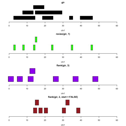
在这一部分,我们使用一个小型的范围来说明一下基因的范围内(intra-range)操作,包括reduce, disjoin与gaps。我们添加链和seqname信息,并显示如想调整大小和侧翼(flank)用于识别TSS和启动子区域,如下所示:

一组简单的范围

1
2
ir <- IRanges(c(3, 8, 14, 15, 19, 34, 40),
width = c(12, 6, 6, 15, 6, 2, 7))

现在我们使用图片形式查看一下ir,以及内部范围(intra-range)操作,如下所示:

1
2
3
4
5
par(mfrow=c(4,1), mar=c(4,2,2,2))
plotRanges(ir, xlim=c(0,60))
plotRanges(reduce(ir), xlim=c(0,60))
plotRanges(disjoin(ir), xlim=c(0,60))
plotRanges(gaps(ir), xlim=c(0,60))

plot of chunk lkir

注:plotRange()函数似乎不在这个包中,网上找到了它的原代码,如下所示:

1
2
3
4
5
6
7
8
9
10
11
12
13
14
plotRanges <- function(x, xlim = x, main = deparse(substitute(x)),
col = "black", sep = 0.5, ...)
{
height <- 1
if (is(xlim, "Ranges"))
xlim <- c(min(start(xlim)), max(end(xlim)))
bins <- disjointBins(IRanges(start(x), end(x) + 1))
plot.new()
plot.window(xlim, c(0, max(bins)*(height + sep)))
ybottom <- bins * (sep + height) - height
rect(start(x)-0.5, ybottom, end(x)+0.5, ybottom + height, col = col, ...)
title(main)
axis(1)
}

reduce(x)函数生成一组不重叠的范围,它覆盖了x中的所有位点。这种操作用于生了你许多转录本的基因模式的复杂性,其中我们可能只想要转录出已知区间的地址,不考虑transcript of residence。

disjoin(x)生成一组覆盖x的所有位置的范围,使得分离输出中的任何范围都不会与x中的任何间隔的端点重叠。这为我们提供了连续间隔最大可能的集合,这些连续间隔在原始间隔集中具有端点的地方被分割开。

gaps(x)产生一组覆盖[start(X),end(X)]中未被x中任何范围覆盖的位置的范围。它能给出编码序列位置和外显子间隔,这可用于枚举内含子。

GRanges的扩展

现在我们添加上染色体与链信息,如下所示:

1
2
library(GenomicRanges)
gir = GRanges(seqnames="chr1", ir, strand=c(rep("+", 4), rep("-",3)))

让我们假设间隔代表基因。下图说明了转录起始位点(绿色)、上游启动子区域(紫色)、下游启动子区域(棕色)的位置,如下所示:

1
2
3
4
5
6
par(mfrow=c(4,1), mar=c(4,2,2,2))
plotGRanges(gir, xlim=c(0,60))
#
plotGRanges(resize(gir,1), xlim=c(0,60),col="green")
plotGRanges(flank(gir,3), xlim=c(0,60), col="purple")
plotGRanges(flank(gir,2,start=FALSE), xlim=c(0,60), col="brown")

plot of chunk dopr

注:plotGRanges的源代码如下所示:

1
2
3
4
5
6
7
8
9
10
11
12
13
14
15
16
17
18
plotGRanges = function (x, xlim = x, col = "black", sep = 0.5, xlimits = c(0,
60), ...)
{
main = deparse(substitute(x))
ch = as.character(seqnames(x)[1])
x = ranges(x)
height <- 1
if (is(xlim, "Ranges"))
xlim <- c(min(start(xlim)), max(end(xlim)))
bins <- disjointBins(IRanges(start(x), end(x) + 1))
plot.new()
plot.window(xlim = xlimits, c(0, max(bins) * (height + sep)))
ybottom <- bins * (sep + height) - height
rect(start(x) - 0.5, ybottom, end(x) + 0.5, ybottom + height,
col = col, ...)
title(main, xlab = ch)
axis(1)
}

请注意,我们不需要采取特殊步骤来处理链中的差异

甲基化微阵列数据的可视化

在我们讨论 SummarizedExperiment applications时,我们输入了由Illumina 450k甲基化微阵列生成的数据。

在这一部分中,我们将介绍如何使用GenomicRanges和Gviz来研究一下在基因水平注释下的甲基化模型。这个思路非常简单:只需从所有样本中提取M值(甲基化与总DNA 比值的基因座特定的估计的log转换),并在选定基因的基因模型中绘制出来,如下所示:

我们回顾一下数据是如何获取和导入的:

1
2
3
4
5
6
7
8
9
library(ArrayExpress)
if (!file.exists("E-MTAB-5797.sdrf.txt")) nano = getAE("E-MTAB-5797")
library(minfi)
pref = unique(substr(dir(patt="idat"),1,17)) # find the prefix strings
raw = read.metharray(pref)
glioMeth = preprocessQuantile(raw) # generate SummarizedExperiment
## [preprocessQuantile] Mapping to genome.
## [preprocessQuantile] Fixing outliers.
## [preprocessQuantile] Quantile normalizing.

这些步骤需要网联,并且需要花几分钟。

一旦我们的会话中有 glioMeth ,需要将以下代码添加到会话中。我们将会介绍它是如何工作的。

1
2
3
4
5
6
7
8
9
10
11
12
13
14
15
16
17
18
MbyGene = function(mset, symbol="TP53", rad=5000) {
# phase 1: annotated GRanges for the gene
require(erma)
require(Gviz)
gmod = suppressMessages(genemodel(symbol)) # erma utility
gseq = as.character(seqnames(gmod)[1])
gmod$transcript = symbol
# phase 2: filter down to the region of interest
mlim = mset[which(seqnames(mset)==gseq),] # restrict to chromosome
# now focus the methylation data to vicinity of gene
d1 = subsetByOverlaps(GRanges(rowRanges(mlim),,, getM(mlim)),
range(gmod)+rad)
# phase 3: use Gviz
plotTracks(list(DataTrack(d1),
GeneRegionTrack(gmod,
transcriptAnnotation="transcript", name=gseq),
GenomeAxisTrack(name=gseq, showTitle=TRUE)))
}

代码表明了三个阶段:获取基因区域,并添加转录本(transcript)注释用于绘制所有外显子的结合;将GenomicRatioSet(继承自

对代码的注释表明了三个阶段:获取基因区并添加用于所有外显子联合的信息性绘图的转录注释;将GenomicRatioSet(继承自RangedSummarizedExperiment)缩小到感兴趣的间隔,这个间隔是由基因模式和rad参数确定;使用Gviz来构建可用于绘图的对象,并绘制出来。

Gviz的详细信息在该包的文档中。现在我们绘制出以基因为中心的图形,如下所示:

1
MbyGene(glioMeth, symbol="TERT")

从上图中我们可以发现这些信息:

  • 基因组背景(以兆(megabase)为单位的染色体和区域)。
  • 感兴趣的基因在单行中的结构,它们表示了表达间隔的联合。
  • 450k针近的位置(蓝色数据点的x坐标)。
  • 甲基化估计中的样本间变异。
  • 所选基因组区域的甲基化变异。

在6x模块中,我们将学习如何使用额外的软件包来创建这种类型的交互式展示,允许我们选择基因并随意放大感兴趣的区域。

脚注

更多的信息可以查看 GenomicRanges 包,以及查阅PLOS Comp Bio上的文献,它是GenomicRanges的作者写的:

http://www.ploscompbiol.org/article/info%3Adoi%2F10.1371%2Fjournal.pcbi.1003118

使用vignettes也能查看这个包的众多功能文档,如下所示:

1
browseVignettes("GenomicRanges")

或者是使用help函数:

1
help(package="GenomicRanges", help_type="html")

对于Bed Tools的用户来说,HelloRanges包对于在BEd和GRanges概念框架之间转换概念非常有用。

参考资料

  1. bioc1_grangeOps.Rmd
  2. IRanges and GRanges